5. Getting Started Guide

5.1. About the Observability Example

Observability Framework includes a C++ example that you can use to evaluate the capabilities of this experimental product. The example is installed in your rti_workspace directory, in the /examples/observability/c++ folder.

This section details how the example is configured and how to run it. When you are ready to test the example, refer to the sections Before Running the Example and Running the Example for instructions.

Important

Observability Framework is an experimental product that includes example configuration files for use with several third-party components (Prometheus, Grafana Loki, and Grafana). This release is an evaluation distribution; use it to explore the new observability features that support Connext applications.

Do not deploy any Observability Framework components in production.

5.1.1. Applications

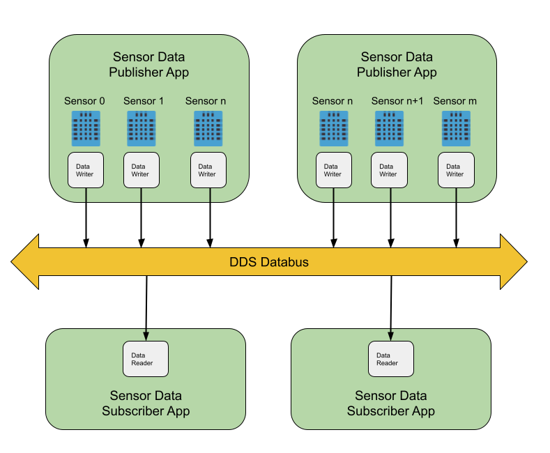
The example consists of two applications:

One application publishes simulated data generated by temperature sensors.
One application subscribes to the sensor data generated by the temperature sensors.

You can run multiple publishing and subscribing applications in the same host, or in multiple hosts, within a LAN. Each publishing application can handle multiple sensors, and each subscribing application subscribes to all sensors.

To learn more about the publish/subscribe model, refer to Publish/Subscribe in the RTI Connext Getting Started Guide.

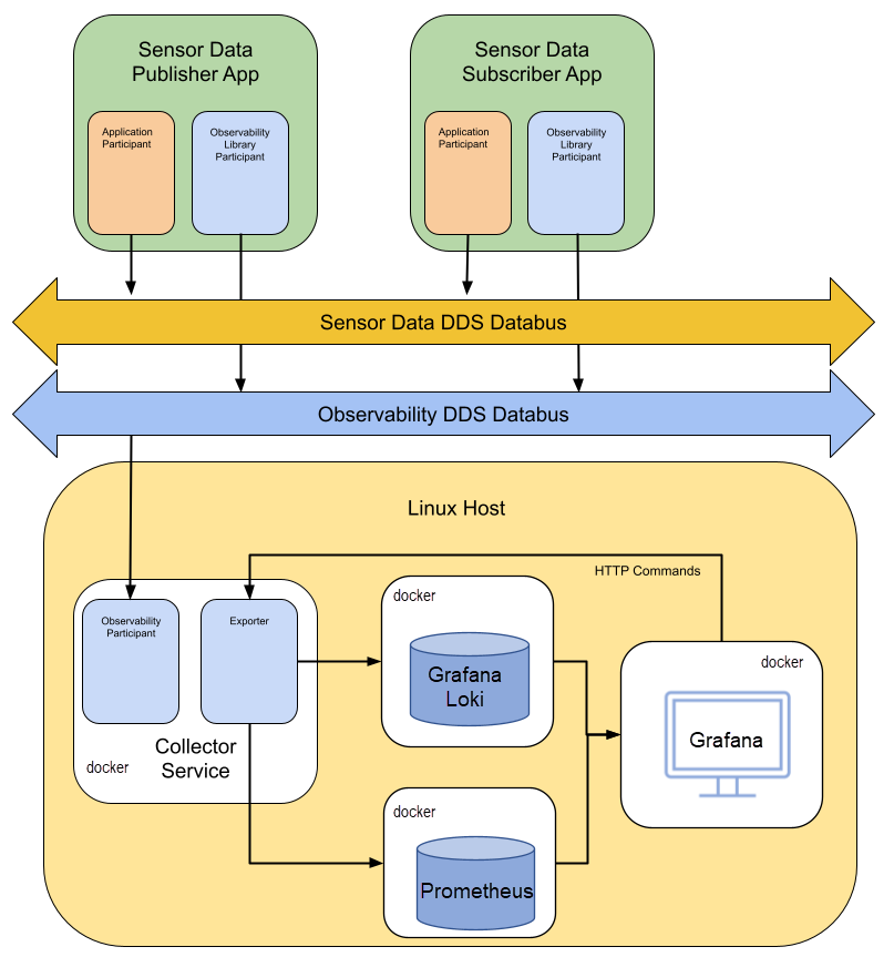
The example applications use Observability Library to distribute telemetry data (logs and metrics) to Observability Collector Service. The collector stores this data in Prometheus (metrics) and Grafana Loki (logs) for analysis and visualization using Grafana.

5.1.2. Data Model

The DDS data model for the Temperature topic used in this example is as follows:

// Temperature data type
struct Temperature {
// ID of the sensor sending the temperature
@key uint32 sensor_id;
// Degrees in Celsius
int32 degrees;
};

Each sensor represents a different instance in the Temperature topic. For general information about data types and topics, refer to Introduction to DataWriters, DataReaders, and Topics and Data Types in the RTI Connext Getting Started Guide.

5.1.3. DDS Entity Mapping

The Publisher application creates one DomainParticipant and n-DataWriters, where n is the number of sensors published by the application. This number is configurable using the command --sensor-count. Each DataWriter publishes one instance. Refer to Keys and Instances in the RTI Connext Getting Started Guide for more information on instances.

The Subscriber application creates one DomainParticipant and a single DataReader to subscribe to all sensor data.

5.1.4. Command Line Parameters

The following command-line switches are available when starting the Publisher and Subscriber applications included in the example. Use this information as a reference when you run the example.

5.1.4.1. Publishing Application

Table 5.1 Publishing Application
Parameter	Data Type	Description	Default
-n, –application-name	<str>	Application name	SensorPublisher_<init_sensor_id>
-d, –domain	<int>	Application domain ID	0
-i, –init-sensor-id	<int>	Initial sensor ID	0
-s, –sensor-count	<int>	Sensor count. Each sensor writes one instance published by a separate DataWriter	1
-o, –observability-domain	<int>	Domain for sending telemetry data	2
-c, –collector-peer	<int>	Collector service peer	localhost
-v, –verbosity	<int>	How much debugging output to show, range 0-3	1

The publishing applications should not publish information for the same sensor IDs. To avoid this issue, you will use the -i command-line parameter to specify the sensor ID to be used as the initial ID when Running the Example.

5.1.4.2. Subscribing Application

Table 5.2 Subscribing Application
Parameter	Data Type	Description	Default
-n, –application-name	<str>	Application name	SensorSubscriber
-d, –domain	<int>	Application domain ID	0
-o, –observability-domain	<int>	Domain for sending telemetry data	2
-c, –collector-peer	<int>	Collector service peer	localhost
-v, –verbosity	<int>	How much debugging output to show, Range 0-3	1

5.2. Before Running the Example

5.2.1. Install Observability Framework

Before running the example make sure that you have installed both the Observability Library and the Collection, Storage and Visualization components. Refer to the Installing and Running Observability Framework section for instructions.

The collection, storage, and visualization components can be installed using one of two methods:

Install the components in a Linux host on the same LAN where the applications run, or
Install the component on a remote Linux host (for example, an AWS instance) reachable over the WAN using RTI Real-Time WAN Transport.

These two methods are described below.

5.2.2. Set Up Environment Variables

After installing Observability Framework, set up the environment variables for running and compiling the example:

Open a command prompt window, if you haven’t already.
Run this script:
$ source <installdir>/resource/scripts/rtisetenv_<architecture>.bash
If you’re using the Z shell, run this:
$ source <installdir>/resource/scripts/rtisetenv_<architecture>.zsh
$ source <installdir>/resource/scripts/rtisetenv_<architecture>.bash
If you’re using the Z shell, run this:
$ source <installdir>/resource/scripts/rtisetenv_<architecture>.zsh
> <installdir>/resource/scripts/rtisetenv_<architecture>.bat

<installdir> refers to the installation directory for Connext.

The rtisetenv script adds the location of the SDK libraries (<installdir>/lib/<architecture>) to your library path, sets the <NDDSHOME> environment variable to point to <installdir>, and puts the RTI Code Generator tool in your path. You may need the RTI Code Generator tool if the makefile for your architecture is not available under the make directory in the example.

Your architecture (such as x64Linux3gcc7.3.0) is the combination of processor, OS, and compiler version that you will use to build your application. For example:

$ source $NDDSHOME/resource/scripts/rtisetenv_x64Linux4gcc7.3.0.bash

5.2.3. Compile the Example

Observability Library can be used in three different ways:

Dynamically loaded: This method requires that the rtimonitoring2 shared library is in the library search path.
Dynamic linking: The application is linked with the rtimonitoring2 shared library.
Static linking: The application is linked with the rtimonitoring2 static library.

You will compile the example using Connext shared libraries so that Observability Library can be dynamically loaded. The example is installed in your rti_workspace directory, in the /examples/observability/c++ folder.

5.2.3.1. Non-Windows Systems

To build this example on a non-Windows system, type the following in a command shell from the example directory:

$ make -f make/makefile_Temperature_<architecture> DEBUG=0

If there is no makefile for your architecture in the make directory, you can generate it using the following rtiddsgen command:

$ rtiddsgen -language C++98 -create makefiles -platform <architecture> -sourceDir src/ -sharedLib -sourceDir src -d ./make ./src/Temperature.idl

5.2.3.2. Windows Systems

To build this example on Windows, open the appropriate solution file for your version of Microsoft Visual Studio in the win32 directory. To use dynamic linking, select Release DLL from the dropdown menu.

5.2.4. Start the Collection, Storage, and Visualization Docker Containers

The Docker containers used for data collection, storage, and visualization can either be run in a Linux host on the same LAN where the applications run or they can be installed on a remote Linux host (for example, an AWS instance) reachable over the WAN using RTI Real-Time WAN Transport.

To run the containers, follow the instructions in the Initialize and Run Docker Containers section.

5.2.4.1. Running on a LAN

Before running the Docker containers used by Observability Framework on a LAN, you must first install a valid Connext Professional license file. This file is required to run Observability Collector Service in a Docker container. For instructions on how to install a license file, see Installing the License File in the RTI Connext Installation Guide.

5.2.4.2. Running on a WAN

Before running the Observability Docker containers on a WAN (for example, in an AWS image) you must first:

Install a valid Connext Anywhere license file. This file is required to run an Observability Collector Service Docker container using RTI Real-Time WAN Transport to enable WAN communications. For instructions on how to install a license file, see Installing the License File in the RTI Connext Installation Guide.
Set the COLLECTOR_PUBLIC_IP environment variable. This variable is the public IP address (reachable over the WAN) of the host running Observability Collector Service.
Set the COLLECTOR_PUBLIC_PORT environment variable. This variable is the public UDP port where Observability Collector Service can be reached. To simplify the example execution, this port must be mapped to the same port number on the host running Observability Collector Service.

Note

Whether running on a LAN or WAN, you can optionally set the OBSERVABILITY_DOMAIN environment variable. This domain ID is used by Observability Collector Service to subscribe to the telemetry data distributed by Observability Library.

If you do not change the domain ID, Observability Collector Service uses domain 2 by default.
If you decide to change the domain ID, you must set the same ID in the applications. Use the command-line parameter --observability-domain upon starting each application.

5.3. Running the Example

Before running the example, select the appropriate values for the following deployment command-line options as needed:

Table 5.3 Optional Command-Line Parameters
Parameter	Description	Default Value
`--observability-domain`	Use this command-line option if you want to overwrite the default domain ID used by Observability Library to send telemetry data to Observability Collector Service.	2
`--collector-peer`	If you run Observability Collector Service in a different host from the applications, use this command-line option to provide the address of the service. For example, 192.168.1.1 (for LAN), or udpv4_wan://10.56.78.89:16000 (for WAN).	localhost

In addition, if you run the applications in different hosts and multicast is not available, use the NDDS_DISCOVERY_PEERS environment to configure the peers where the applications run.

For simplicity, the instructions in this section assume that you are running the applications and the Docker containers used by Observability Framework on the same host with the default observability domain.

5.3.1. Start the Applications

This example assumes x64Linux4gcc7.3.0 as the architecture.

In a new browser window, go to http://localhost:3000 and log in using your Grafana dashboard credentials.

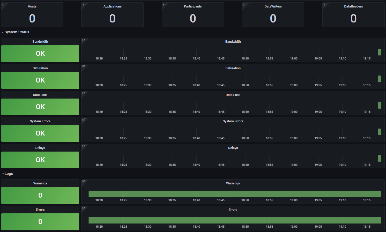
Note that at this point, no DDS applications are running.

From the example directory, open two terminals and start two instances of the application that publishes temperature sensor data. The command and resulting output for each instance are shown below. The -i parameter specifies the sensor ID that will be used. The -n parameter assigns a name to the application. You will use this name to send commands in Change the Application Logging Verbosity.

The first instance creates two sensors.

$ ./objs/x64Linux4gcc7.3.0/Temperature_publisher -n SensorPublisher_1
-d 57 -i 0 -s 2 -v 2
**********************************************************
******** Temperature Sensor Publisher App ****************
**********************************************************

Running with parameters:
   Application Resource Name: /applications/SensorPublisher_1
   Domain ID: 57
   Init Sensor ID: 0
   Sensor Count: 2
   Observability Domain: 2
   Collector Peer: udpv4://localhost
   Verbosity: 2
Command>

The second instance creates one sensor.

$ ./objs/x64Linux4gcc7.3.0/Temperature_publisher -n SensorPublisher_2
-d 57 -i 2 -s 1 -v 2
*********************************************************
******** Temperature Sensor Publisher App ***************
*********************************************************

Running with parameters:
   Application Resource Name: /applications/SensorPublisher_2
   Domain ID: 57
   Init Sensor ID: 2
   Sensor Count: 1
   Observability Domain: 2
   Collector Peer: udpv4://localhost
   Verbosity: 2
Command>

From the example directory, open a new terminal and start one instance of the application that subscribes to temperature sensor data.

$ ./objs/x64Linux4gcc7.3.0/Temperature_subscriber -n SensorSubscriber
   -d 57 -v 2
**********************************************************
******** Temperature Sensor Subscriber App ***************
**********************************************************

Running with parameters:
   Application Resource Name: /applications/SensorSubscriber
   Domain ID: 57
   Observability Domain: 2
   Collector Peer: udpv4://localhost
   Verbosity: 2
Command>

Note

The two Publisher applications and the Subscriber application are started with verbosity set to WARNING (-v 2). You may see any of the following warnings on the console output. These warnings are expected.

WARNING [0x01017774,0xFF40EEF6,0xEC566CA8:0x000001C1{Domain=2}|ENABLE|LC:DISC]NDDS_Transport_UDPv4_Socket_bind_with_ip:0X1EE6 in use
WARNING [0x01017774,0xFF40EEF6,0xEC566CA8:0x000001C1{Domain=2}|ENABLE|LC:DISC]NDDS_Transport_UDPv4_SocketFactory_create_receive_socket:invalid port 7910
WARNING [0x01017774,0xFF40EEF6,0xEC566CA8:0x000001C1{Domain=2}|ENABLE|LC:DISC]NDDS_Transport_UDP_create_recvresource_rrEA:!create socket
WARNING [0x010175D0,0x7A41F985,0xF3813392:0x000001C1{Name=Temperature DomainParticipant,Domain=57}|ENABLE|LC:DISC]NDDS_Transport_UDPv4_Socket_bind_with_ip:0X549C in use
WARNING [0x010175D0,0x7A41F985,0xF3813392:0x000001C1{Name=Temperature DomainParticipant,Domain=57}|ENABLE|LC:DISC]NDDS_Transport_UDPv4_SocketFactory_create_receive_socket:invalid port 21660
WARNING [0x010175D0,0x7A41F985,0xF3813392:0x000001C1{Name=Temperature DomainParticipant,Domain=57}|ENABLE|LC:DISC]NDDS_Transport_UDP_create_recvresource_rrEA:!create socket
WARNING [0x010175D0,0x7A41F985,0xF3813392:0x000001C1{Name=Temperature DomainParticipant,Domain=57}|ENABLE|LC:DISC]DDS_DomainParticipantDiscovery_add_peer:no peer locators for: peer descriptor(s) = "builtin.shmem://", transports = "", enabled_transports = ""

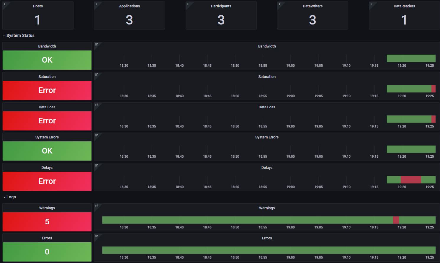
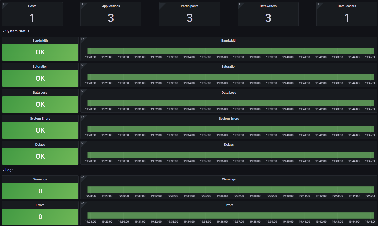
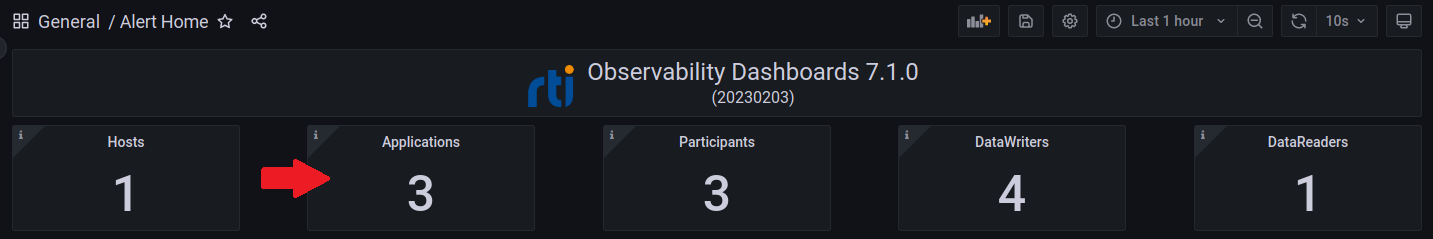
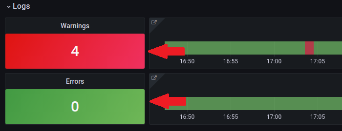
Your Grafana dashboard should now provide information about the new Hosts, Applications, and DDS entities (Participants, DataWriters, and DataReaders). There should be 1 Host, 3 Applications, 3 Participants, 3 DataWriters, and 1 DataReader.

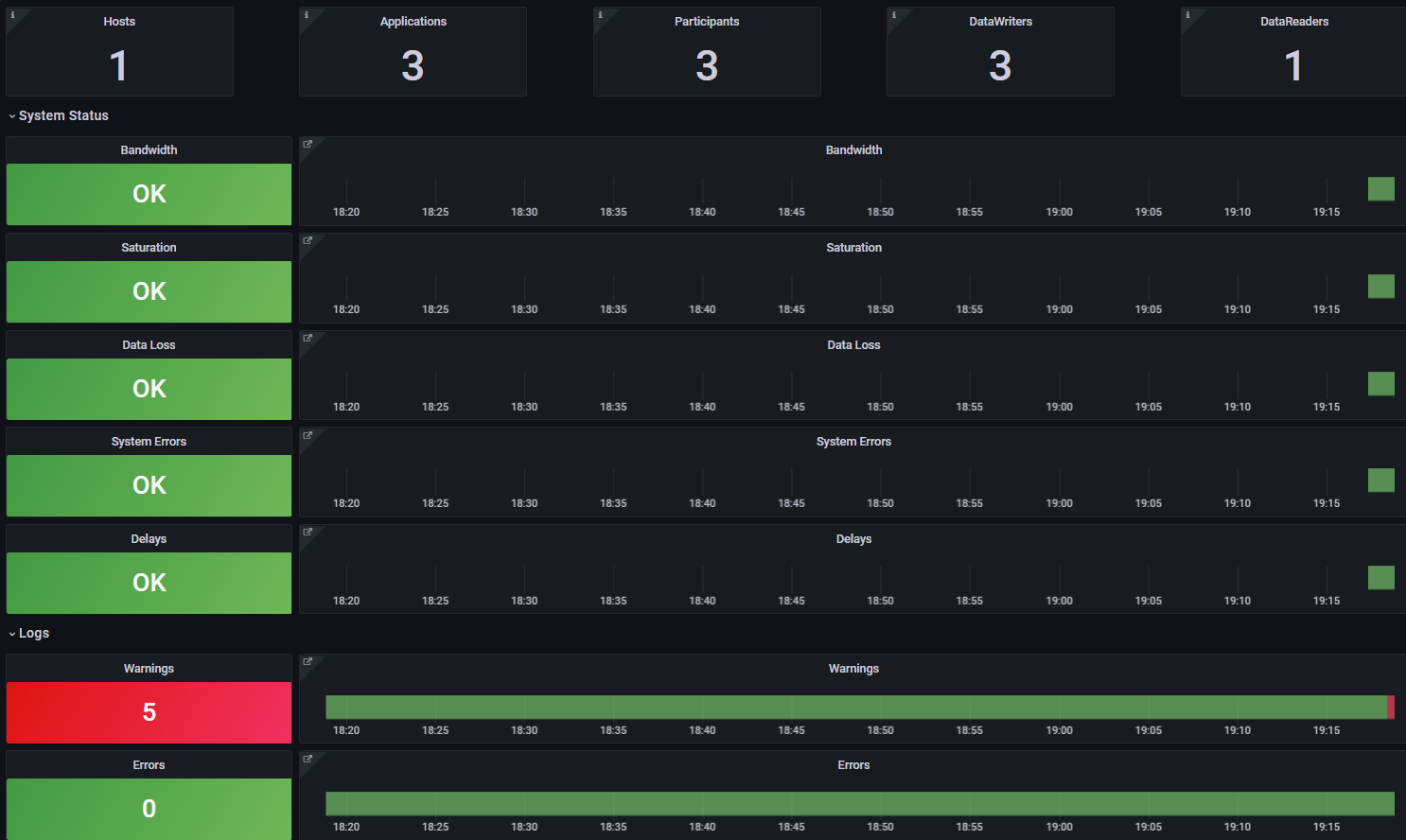
The Grafana main dashboard pictured above indicates that the system is healthy. The warnings in the log section are expected and related to the reservation of communication ports. You can select the Warnings panel to visualize them.

Next, you will introduce different failures that will affect the system’s health.

5.3.2. Changing the Time Range in Dashboards

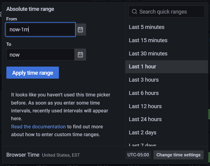
While running the examples, you can change the time range in the dashboards to reduce or expand the amount of history data displayed. Use the time picker dropdown at the top right to change the time range in any dashboard.

The time picker includes a predefined list of time ranges to choose from. If you want to use a custom time range, enter the desired range in the From field. Use the format “now-< custom time >,” where < custom time > is a unit of time; Grafana supports m-minute, h-hour, and d-day time units. For example, to show a custom range of one minute, enter “now-1m” in the From field, then select Apply Time Range.

Note

The time range may be changed on any dashboard, but all changes are temporary and will reset to 1 hour when you return to the Alert Home dashboard. Changes to the time range made in the Alert Home dashboard are unique in that the selected time range will be propagated to other dashboards as you navigate through the hierarchy.

5.3.3. Simulate Sensor Failure

The DataWriters in each application are expected to send sensor data every second, and the DataReader expects to receive sensor data from each sensor every second. This QoS contract is enforced with the Deadline QoS Policy set in USER_QOS_PROFILES.xml. Refer to Deadline QoS Policy in the RTI Connext Getting Started Guide for basic information, or DEADLINE QoSPolicy in the RTI Connext Core User’s Manual for detailed information.

<deadline>
   <period>
      <sec>1</sec>
      <nanosec>0</nanosec>
   </period>
</deadline>

To simulate a failure in the sensor with ID 0, enter the following command in the first Temperature_publisher instance:

Command> stop 0

The Grafana dashboard updates to indicate the sensor failure. The dashboard does not update immediately; you may have to wait a few seconds to see the change reflecting the sensor failure as a Delay error. That error is expected because the deadline policy was violated when you stopped the sensor with ID 0.

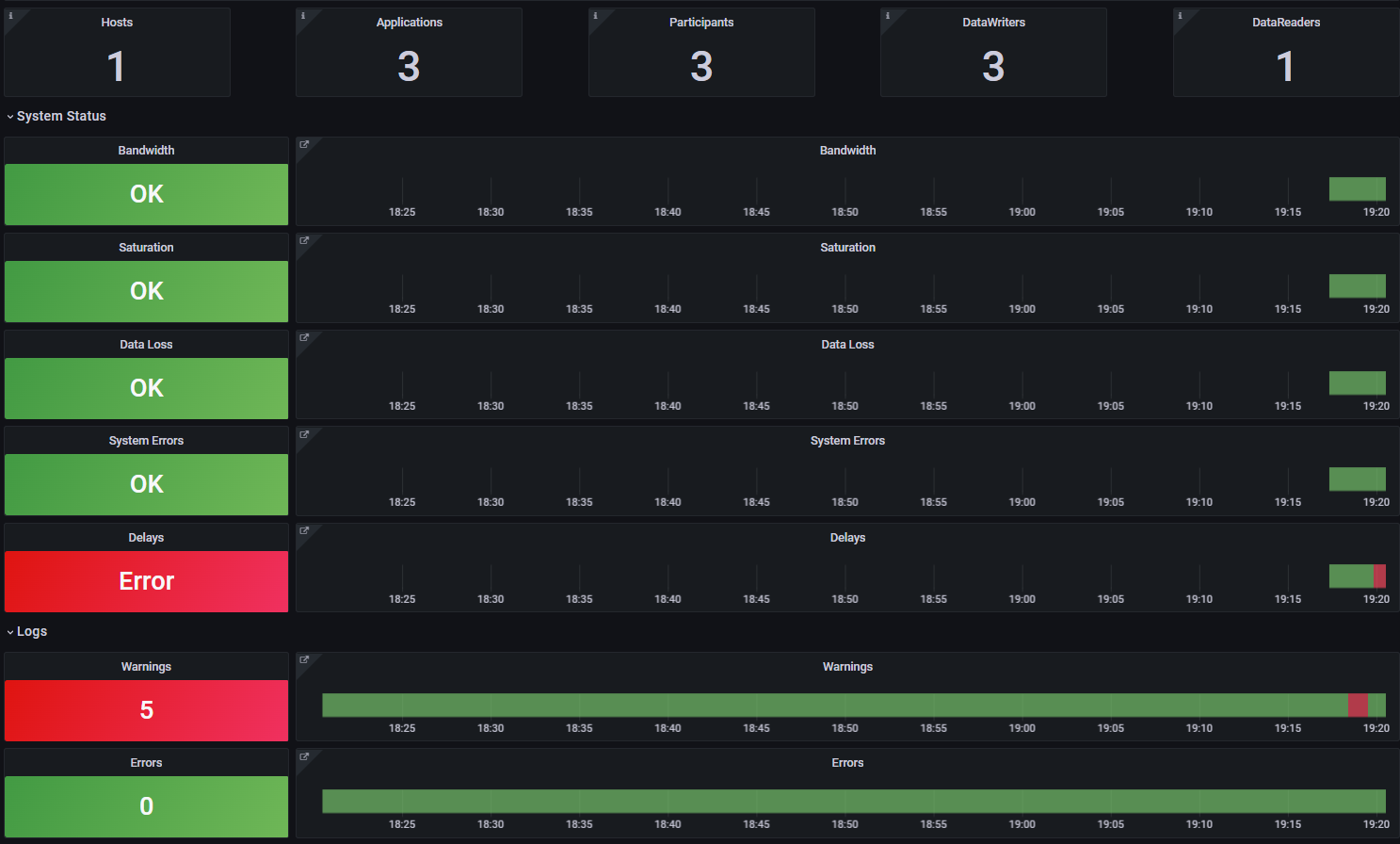
The Grafana dashboards are hierarchical. Now that you know something is happening related to latency (or delays), you can get additional details to determine the root cause. Select the Delays panel to drill down to the next level and get more information about the error.

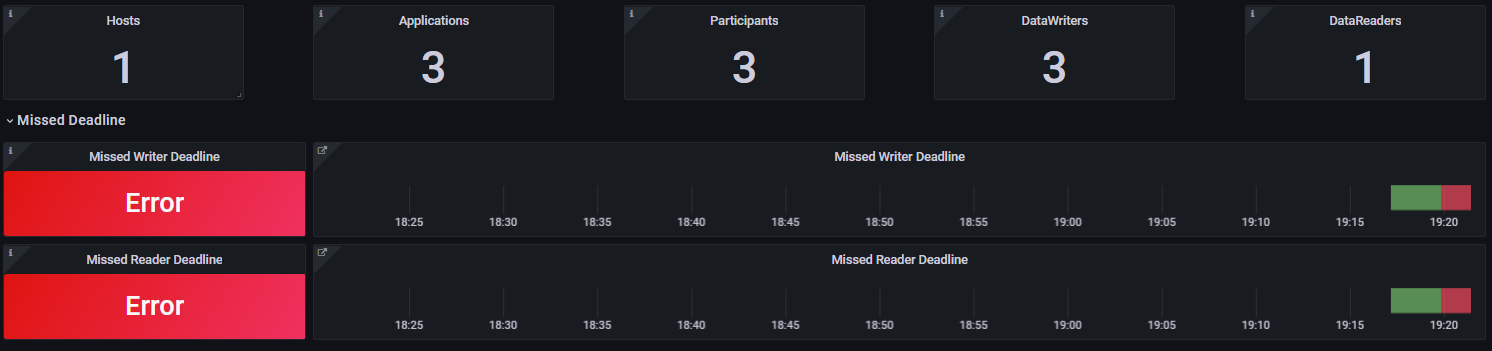
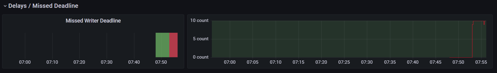
The second level of the Grafana dashboard indicates that there were deadline errors, which were generated by both the DataWriters associated with the sensors and the DataReader expecting sensor data at a specific rate. Still, we do not know which sensor the problem originated from. To determine that, we have to go one level deeper; select the Missed Writer Deadline panel to see which DataWriter caused the problem.

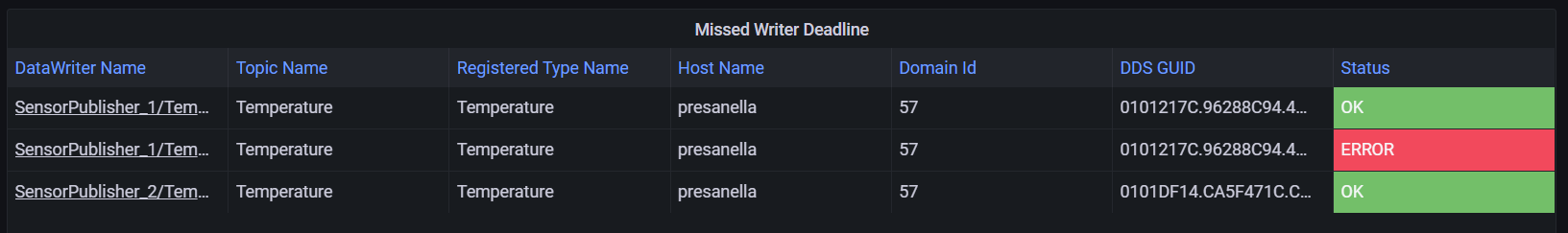
The third level of the Grafana dashboard provides a list of entities providing deadline information. In this case we see three entities, or DataWriters, each associated with a sensor. We also see the first entity is failing. But what sensor does that entity represent?

Looking at the DataWriter Name column, we can see that the failing sensor has the name “Sensor with ID=0”. This name is set using the EntityName QoS Policy when creating a DataWriter. If you want additional information, such as the machine where the sensor DataWriter is located, select the Sensor with ID-0 link in the DataWriter Name column.

The fourth and last level of the Grafana dashboard provides detailed information about an individual entity, including location-related information such as Host Name and Process Id.

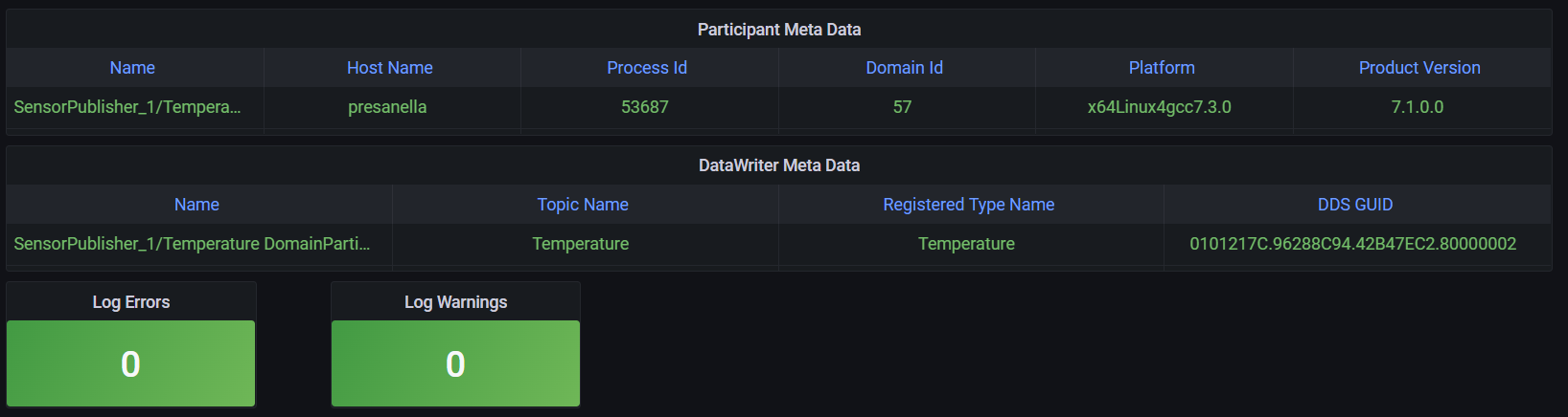
In addition, this last level provides information about individual metrics for the entity. Scroll down to see the details of the missed deadline metric.

Next, restore the health of the failing sensor to review how the dashboard changes. Restart the first Temperature_publisher instance using the command start 0.

Command> start 0

Go back to the Alert Home dashboard to confirm that the sensor becomes healthy. After a few seconds, the Delays panel should indicate the sensor is healthy. However, part of the Delay panel is still red. Depending on the selected dashboard time range, the sensor was likely unhealthy for part of the time displayed..

5.3.4. Simulate Slow Sensor Data Consumption

A subscribing application can be configured to consume sensor data at a lower rate than the publication rate. In a real scenario, this could occur if the subscribing application becomes CPU bound.

This scenario simulates a problem with the subscribing application; a bug in the application logic makes it slow in processing sensor data. To test this failure, enter the slow_down command in the Temperature_subscriber instance:

Command> slow_down

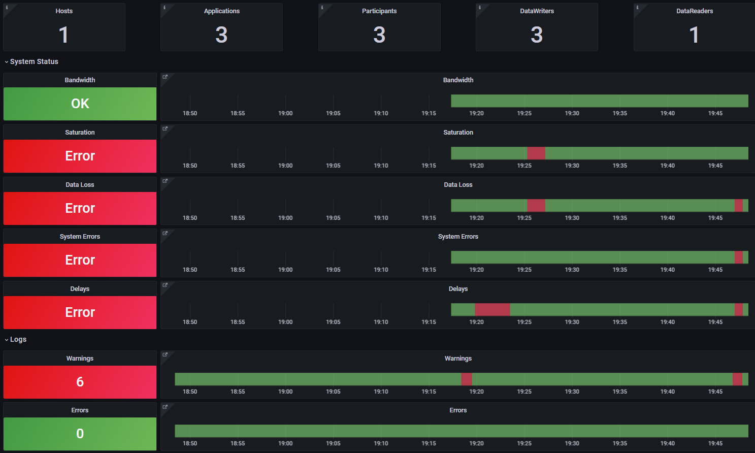
After some seconds, the Grafana dashboard displays two new system errors related to saturation and unexpected data losses. Because the DataReader is not able to keep up with the sensor data, the dashboard indicates that there are potential data losses. At the same time, being unable to keep up with the sensor data could be a saturation sign. For example, the DataReader may consume 100% of the CPU due to the application bug.

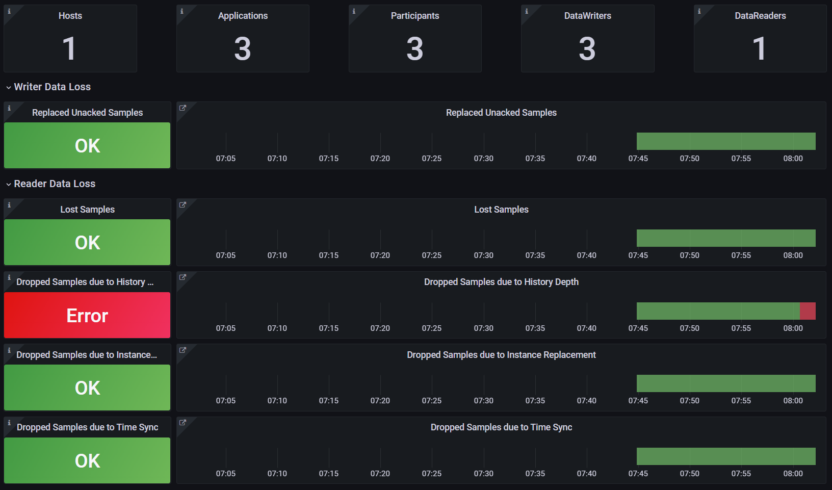
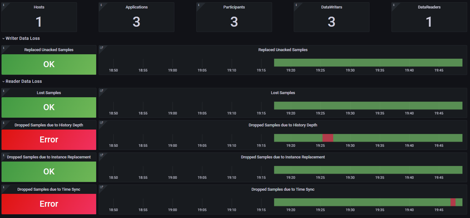
As you did when testing the sensor failure, select the displayed errors to navigate the dashboard hierarchy and determine the root cause of the problem. To go to the second level, select the Data Loss panel to see the reason for the losses. Because you slowed the subscriber application, the DataReader is not able to read fast enough. The Dropped Samples due to History Depth metric reveals the type of failure. Select the red errors to drill down and review further details about the problem.

Grafana dashboard slow sensor error level 2

After reviewing the errors, restore the health of the failing DataReader. In the Temperature_subscriber application, enter the speed_up command.

Command> speed_up

In Grafana, go back to the home dashboard and wait until the system becomes healthy again. After a few seconds, the Saturation and Data Loss panels should indicate a healthy system. Also, adjust the time window to one minute and wait until all the system status panels are green again.

5.3.5. Simulate Time Synchronization Failures

The DataReaders created by the subscribing applications expect that clocks are synchronized. The source timestamp associated with a sensor sample by the Publisher should not be farther in the future from the reception timestamp than a configurable tolerance. This behavior is configured using the DestinationOrder QoS Policy set in USER_QOS_PROFILES.xml.

<destination_order>
   <kind>BY_SOURCE_TIMESTAMP_DESTINATIONORDER_QOS</kind>
   <source_timestamp_tolerance>
      <sec>1</sec>
      <nanosec>0</nanosec>
   </source_timestamp_tolerance>
</destination_order>

This final simulation demonstrates how to use logging information to troubleshoot problems. In this scenario, you’ll create a clock synchronization issue in the first instance of Temperature_publisher. The clock will move forward in the future by a few seconds, causing the DataReader to drop some sensor samples from the publishing application.

To simulate this scenario, enter clock_forward 0 in the first Temperature_publisher instance.

Command> clock_forward 0

After some seconds, three panels in the system status section will turn red: Data Loss, System Errors, and Delays. Each is affected by the same underlying problem. You can select the red errors to drill down through the dashboard hierarchy and determine the root cause of the problem.

First, select the Data Loss panel to see the reason for the error. The DataReader dropped samples coming from one or more of the DataWriters due to time synchronization issues.

This error indicates that the DataReader in the subscribing application dropped some samples, but can’t yet identify the problem sensor or DataWriter. To determine that, select the Dropped Samples due to Time Sync panel.

Grafana dashboard time sync error level 2

At this level, you can locate the DataReader reporting the error, but not the DataWriter causing it. Select the TemperatureSensor link in the DataReader Name column to go one more level down.

Grafana dashboard time sync error level 3

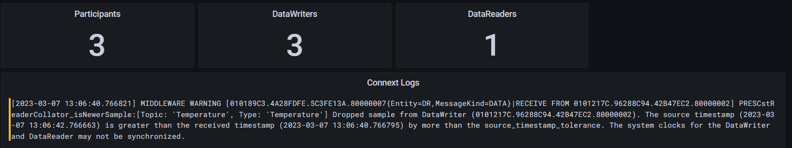
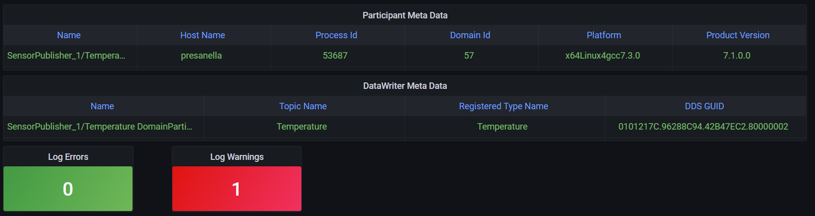
On the endpoint dashboard, there is one log warning associated with the DataReader reporting time synchronization issues. Select the red Log Warning to view the warning message logged by the DataReader.

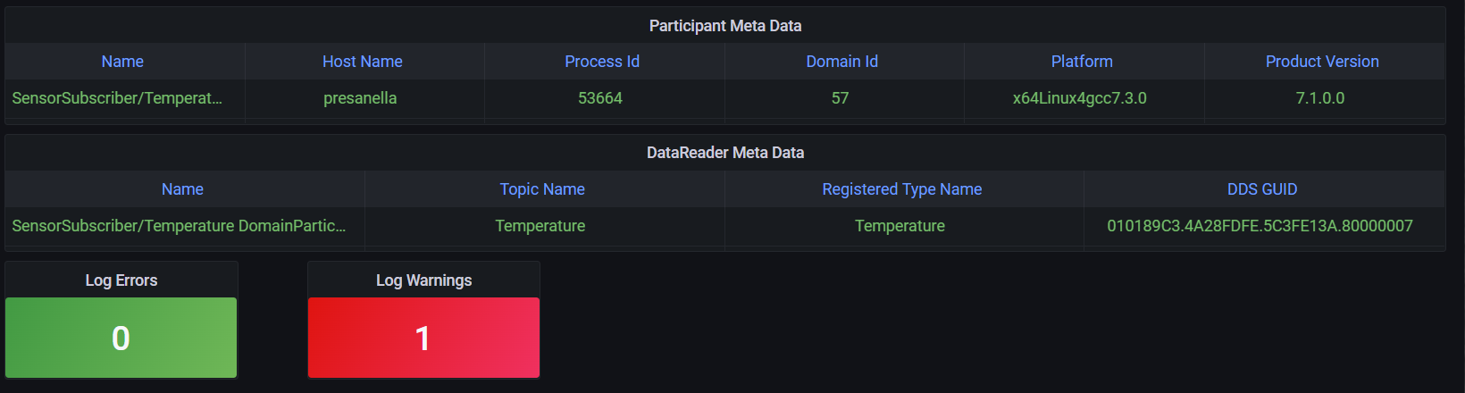
Grafana dashboard time sync error level 4

This warning message provides information about the GUID of the DataWriter that published the sensor data that was dropped due to time synchronization issues. But how do we locate the DataWriter from its GUID?

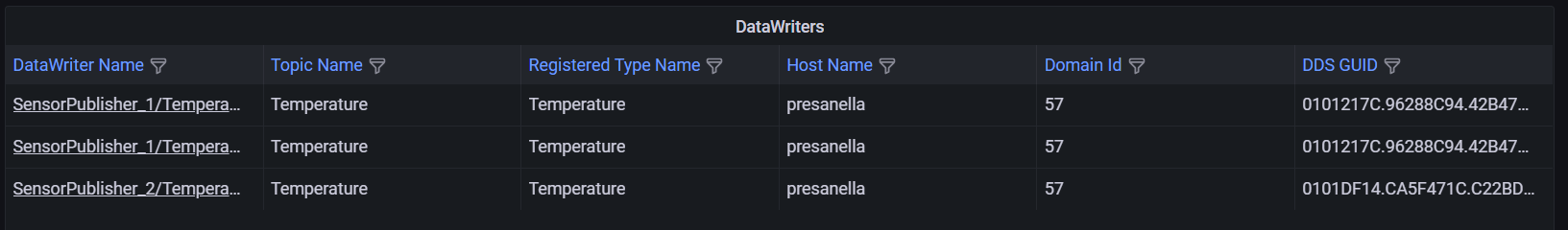
Select the DataWriters panel to view a list of the running DataWriters.

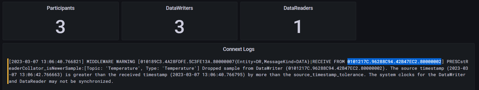
Grafana dashboard time sync error warning

Note the highlighted RECEIVE FROM GUID in the log message. This represents the corresponding DataWriter that created the warning. (You can copy this GUID at this point).

Grafana dashboard time sync error warning highlightes

Now that we have a list of DataWriters, we can compare their GUIDs with the GUID in the log message to find the problem DataWriter. In this case the list does not have a lot of entries, so you can search manually.

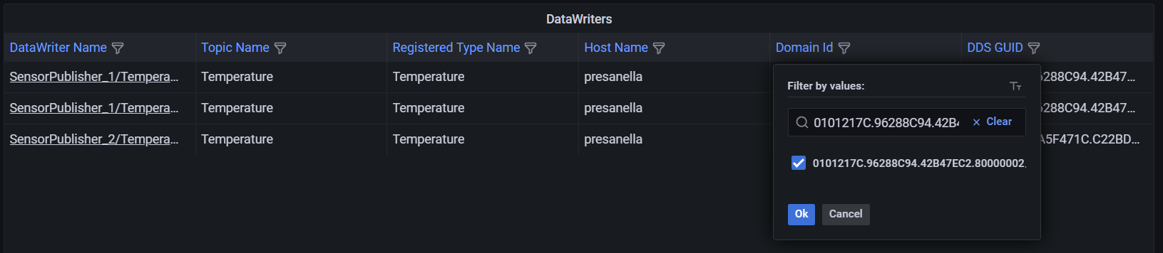
However, when the number of entries is large, you can click on the funnel icon next to the GUID label to filter the list to the one writer with time synchronization issues by typing in the GUID or pasting the value copied from teh log message.

Finally, select the problem DataWriter to learn its identity.

The problem DataWriter corresponds to sensor 0. You have successfully done root cause analysis by correlating metrics and logging.

5.3.6. Change the Application Logging Verbosity

Observability Library has two verbosity settings.

Collection verbosity controls what level of log messages an application generates.
Forwarding verbosity controls the level of log messages an application forwards to the Observability Collector Service (making the messages visible in the dashboard).

By default, Observability Library only forwards error and warning log messages, even if the applications generate more verbose logging. Forwarding messages at a higher verbosity for all applications may saturate the network and the different Observability Framework components, such as Observability Collector Service and the logging aggregation backend (Grafana Loki in this example).

However, in some cases you may want to change the logging Collection verbosity and/or the Forwarding verbosity for specific applications to obtain additional information when doing root cause analysis.

In this section you will increase both the Collection and Forwarding verbosity level for the first publishing application. To do that, you will use the application resource name generated by using the -n command-line option. The three applications have the following names:

/applications/SensorPublisher_1
/applications/SensorPublisher_2
/applications/SensorSubscriber

To change the Collection verbosity:

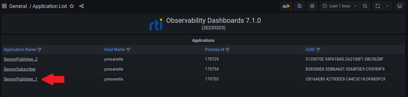
From the Alert Home dashboard, select the Applications indicator to open the Application List dashboard.
From the Application List dashboard, select the SensorPublisher_1 link to open the Alert Application Status dashboard.
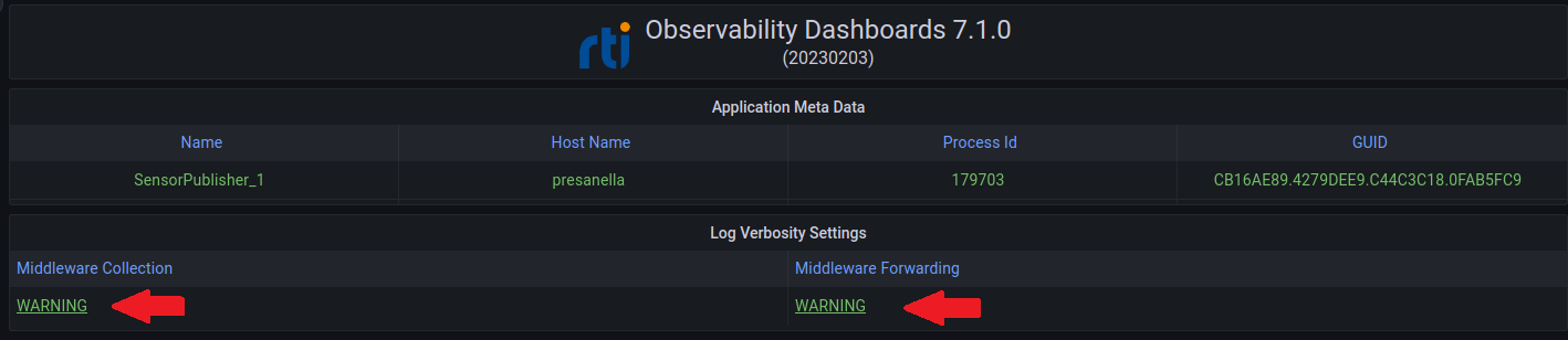
From the Alert Application Status dashboard, select the Middleware Collection log verbosity to open the Log Control dashboard.
From the Log Control dashboard, select DEBUG from the Log Collection Verbosity drop down menu.

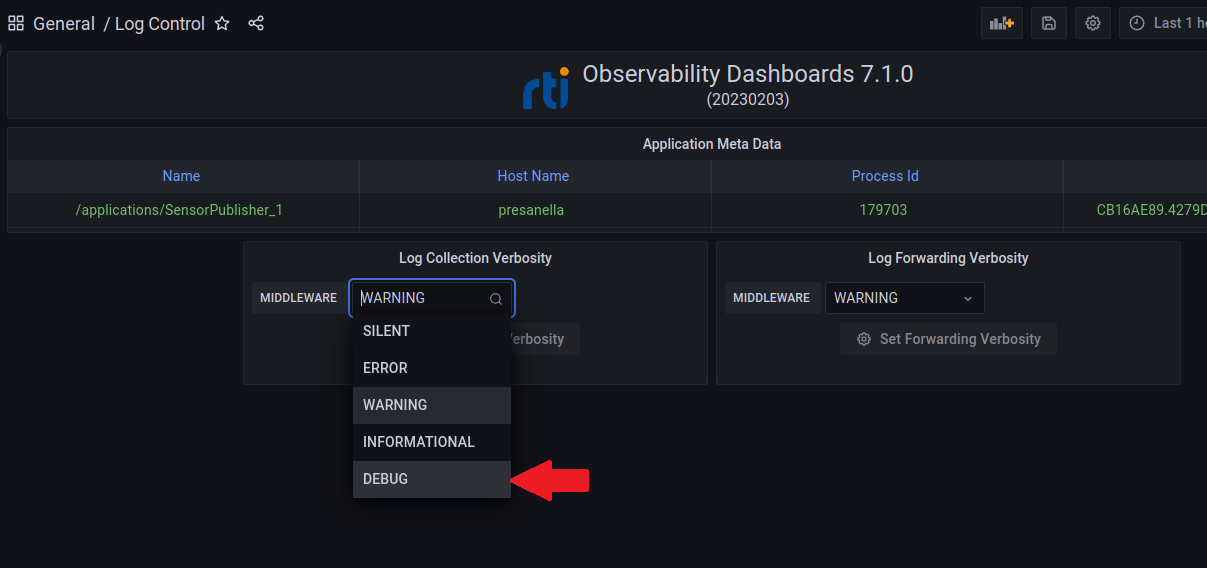
Note that the verbosity setting color changes to yellow, indicating a change has been made. Also, the Set Collection Verbosity button is blue and enabled.
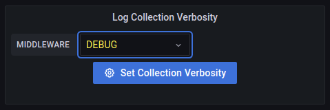
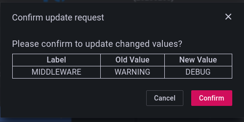
Select the Set Collection Verbosity button. When prompted to confirm the change, select Confirm to set the Collection Verbosity level to DEBUG at the application.

The application Collection verbosity is now DEBUG. If you examine the terminal window for SensorPublisher_1, you will see something similar to the following.

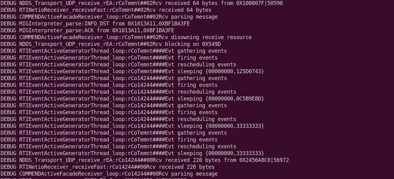
Observability application debug messages

At this point, the SensorPublisher_1 application is generating log messages at the DEBUG level as shown in the terminal window, but the log messages are not being forwarded to Observability Collector Service because the Forwarding Verbosity is still at WARNING.

To set the logging Forwarding verbosity to DEBUG, repeat steps 4 - 5 above using the Log Fowarding Verbosity pull down.

After setting both the Collection and Forwarding verbosity to DEBUG, you should see DEBUG messages for the SensorPublisher_1 application in the Log Dashboard. To view the Log Dashboard, click the Home icon to go back to the Alert Home dashboard.

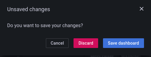
Note

If you are using the dashboards as an admin user, you will be prompted to save your changes. Select the Discard button; the changes to the dashboard do not need to be saved, since they are set in the application. This prompt does not appear when running with lesser permissions.

Now that both Collection and Forwarding verbosity are set to DEBUG, you can configure the Log Dashboard to display DEBUG log messages.

From the Alert Home dashboard, in the Logs section, select either the Warnings or Errors indicator to open the Log Dashboard.
From the Log Dashboard, in the Filter Log Level dropdown, select the DEBUG checkbox.

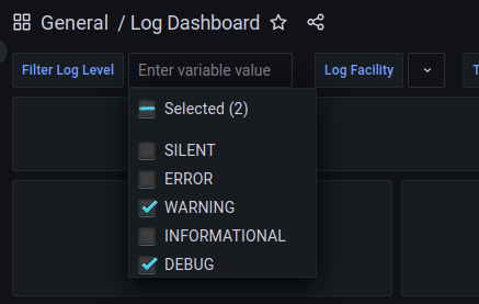
Once DEBUG is added to the Filter Log Level, DEBUG log messages appear in the Connext Logs panel.

You can manipulate the Log Control settings to verify application and dashboard behavior as shown in Table 5.4.

Table 5.4 Collection and Forwarding Log Verbosity DEBUG Behavior
Collection Verbosity	Forwarding Verbosity	Application DEBUG Log Output	Grafana Connext DEBUG Logs
WARNING	WARNING	NO	NO
DEBUG	WARNING	YES	NO
WARNING	DEBUG	NO	NO
DEBUG	DEBUG	YES	YES

5.3.7. Close the Applications

When done working with the example, enter quit in each running application to shut it down.